
Where a career exists can matter almost as much as what it pays. An occupation concentrated in a few states may offer a strong market to workers who can relocate and a much narrower one to workers who cannot. An occupation spread across the country may reduce dependence on any single regional economy.
MyTopMatch examined this question using the newest annual state Occupational Employment and Wage Statistics files listed by the U.S. Bureau of Labor Statistics as of September 8, 2026: the May 2025 release. [1] The study measured geographic diversification across the 50 states and the District of Columbia while preserving suppressed or unavailable state cells as missing.
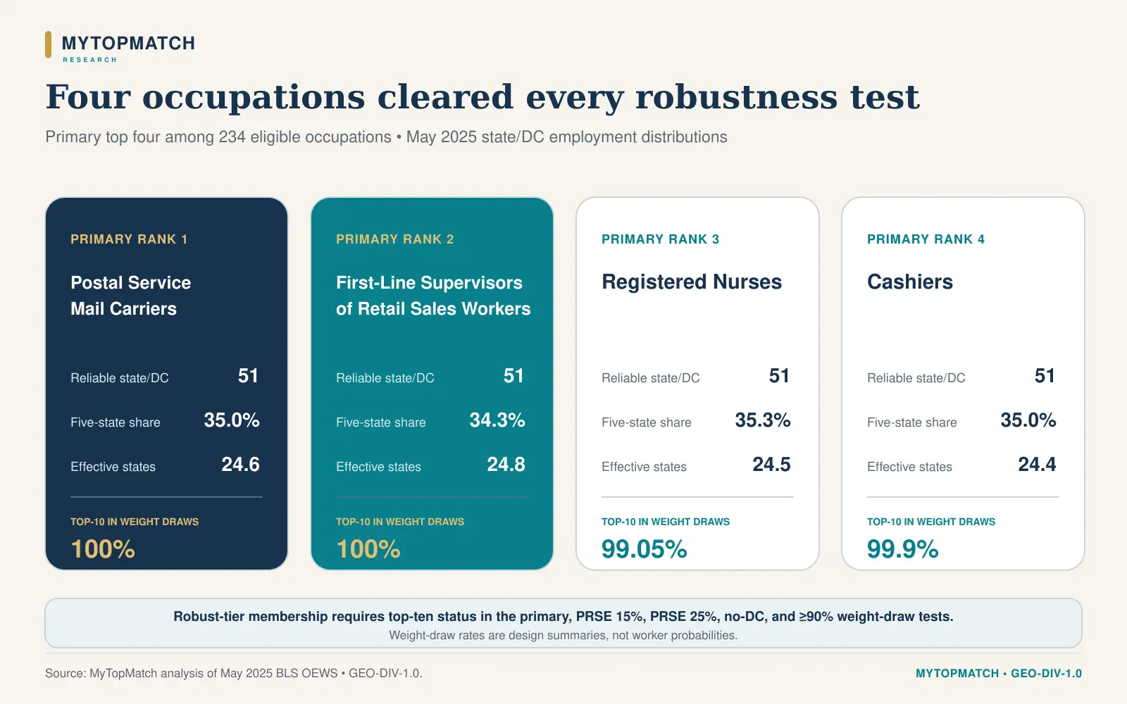
Four occupations formed the most robust tier in the analysis: Postal Service Mail Carriers; First-Line Supervisors of Retail Sales Workers; Registered Nurses; and Cashiers. They occupied the top four positions in the primary specification and remained in the top ten under every reliability, geography, and weighting test required for the robust-tier label.
The result is narrower than a list of the “best careers anywhere.” OEWS measures existing wage-and-salary employment in nonfarm establishments. It does not count current job advertisements or estimate a person's likelihood of being hired. [4]
The finding at a glance
| Occupation | Primary rank | National employment | Reliable state/DC estimates | Five-state share | Effective states | Similarity to all-jobs distribution | Top-ten inclusion in weight draws |
|---|---|---|---|---|---|---|---|
| Postal Service Mail Carriers | 1 | 328,820 | 51 | 35.0% | 24.6 | 94.4% | 100.0% |
| First-Line Supervisors of Retail Sales Workers | 2 | 1,121,800 | 51 | 34.3% | 24.8 | 93.0% | 100.0% |
| Registered Nurses | 3 | 3,379,720 | 51 | 35.3% | 24.5 | 95.1% | 99.05% |
| Cashiers | 4 | 3,089,410 | 51 | 35.0% | 24.4 | 94.4% | 99.9% |
Source data — May 2025 BLS OEWS national and state cross-industry employment estimates. [1][2][3] Derived calculations: MyTopMatch reliable-state counts, five-state shares, effective-state values, all-jobs distribution similarity, component percentiles, composite scores, ranks, and sensitivity summaries. Statistical findings: No population hypothesis test or causal model is used. Weight and threshold checks evaluate the stability of the derived ranking under alternative analytical choices. Interpretation: The four occupations have broad state-level employment footprints in this edition. That breadth may reduce dependence on a small number of states, but it does not prove that openings, wages, access, or job quality are favorable.
What “geographically diversified” means here
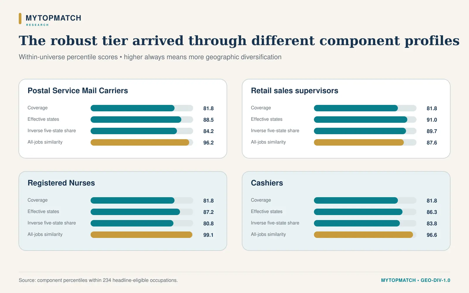
Geographic diversification is not a single observable variable. MyTopMatch defined it using four complementary components:
- Reliable-state coverage. The share of the 50 states and District of Columbia with a published employment estimate and employment PRSE no greater than 20%.
- Effective states. The inverse Herfindahl-Hirschman Index of reliable state employment shares. If employment were divided equally across k states, the measure would equal k. It is an index-equivalent, not a literal count of places with jobs.
- Inverse five-state share. The share of reliable-state employment found in the five largest state counts, scored so that a lower concentration receives a higher diversification score.
- Similarity to the all-jobs state distribution. One minus the total-variation distance between an occupation's reliable-state employment distribution and the all-occupation employment distribution across the same observed states.
The components answer different questions. Effective states and the five-state share reward a flatter distribution. The all-jobs comparison asks whether an occupation follows the broad shape of the national labor market, recognizing that California, Texas, Florida, New York, and other large states naturally employ more people.
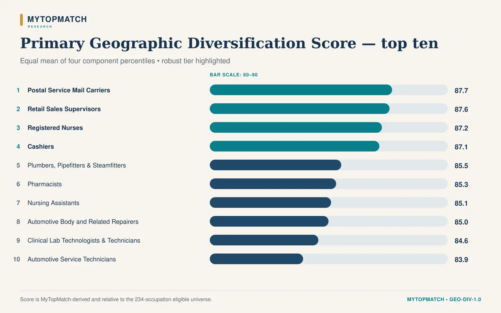
Each component was percentile-ranked within the eligible occupation universe. The primary Geographic Diversification Score is the equal mean of the four percentile scores. Scores are relative to the 234 eligible occupations and should not be compared across future editions unless the universe and method remain fixed.
The primary top ten
| Rank | Occupation | Score | Reliable state/DC estimates | Five-state share | Effective states |
|---|---|---|---|---|---|
| 1 | Postal Service Mail Carriers | 87.7 | 51 | 35.0% | 24.6 |
| 2 | First-Line Supervisors of Retail Sales Workers | 87.6 | 51 | 34.3% | 24.8 |
| 3 | Registered Nurses | 87.2 | 51 | 35.3% | 24.5 |
| 4 | Cashiers | 87.1 | 51 | 35.0% | 24.4 |
| 5 | Plumbers, Pipefitters, and Steamfitters | 85.5 | 51 | 34.6% | 24.6 |
| 6 | Pharmacists | 85.3 | 51 | 35.4% | 24.3 |
| 7 | Nursing Assistants | 85.1 | 51 | 31.2% | 27.8 |
| 8 | Automotive Body and Related Repairers | 85.0 | 51 | 35.2% | 24.3 |
| 9 | Clinical Laboratory Technologists and Technicians | 84.6 | 51 | 34.4% | 24.8 |
| 10 | Automotive Service Technicians and Mechanics | 83.9 | 51 | 35.0% | 24.3 |
The exact order is a model result rather than an official BLS ranking. It combines MyTopMatch-defined components and weights. The robust-tier finding therefore requires more than appearing in this one table.
Why the robust tier contains four occupations
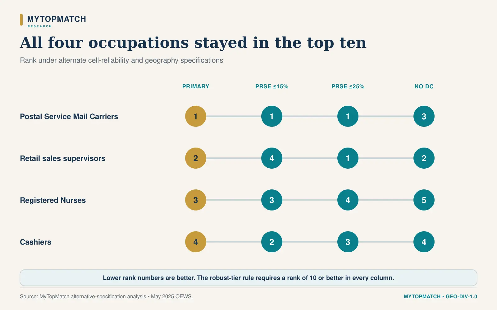
The four tier members met every rule below:
- top ten in the primary equal-weight specification;
- top ten when the employment PRSE ceiling was tightened from 20% to 15%;
- top ten when the ceiling was relaxed to 25%;
- top ten when the District of Columbia was removed; and
- top-ten inclusion in at least 90% of 2,000 reasonable weight draws.
Their alternate ranks were:
| Occupation | PRSE <=15% | PRSE <=25% | DC excluded | Weight-draw rank, 5th-95th percentile |
|---|---|---|---|---|
| Postal Service Mail Carriers | 1 | 1 (tie) | 3 | 1-4 |
| First-Line Supervisors of Retail Sales Workers | 4 | 1 (tie) | 2 | 1-4 |
| Registered Nurses | 3 | 4 | 5 | 1-8 |
| Cashiers | 2 | 3 | 4 | 3-6 |
Other occupations performed strongly in the primary table but moved outside the top ten under at least one required test or failed the 90% weight-inclusion rule. This does not make those careers geographically narrow. It means the evidence for placing them in the most robust tier was weaker under the frozen standard.
Across all 234 occupations, the alternative rank correlations with the primary specification were 0.993 when DC was excluded and 0.980 when the PRSE ceiling was 25%. The stricter 15% analysis retained 185 overlapping occupations and had a rank correlation of 0.971. Each alternative retained eight of the primary top ten.
A direct metric reveals a different leader
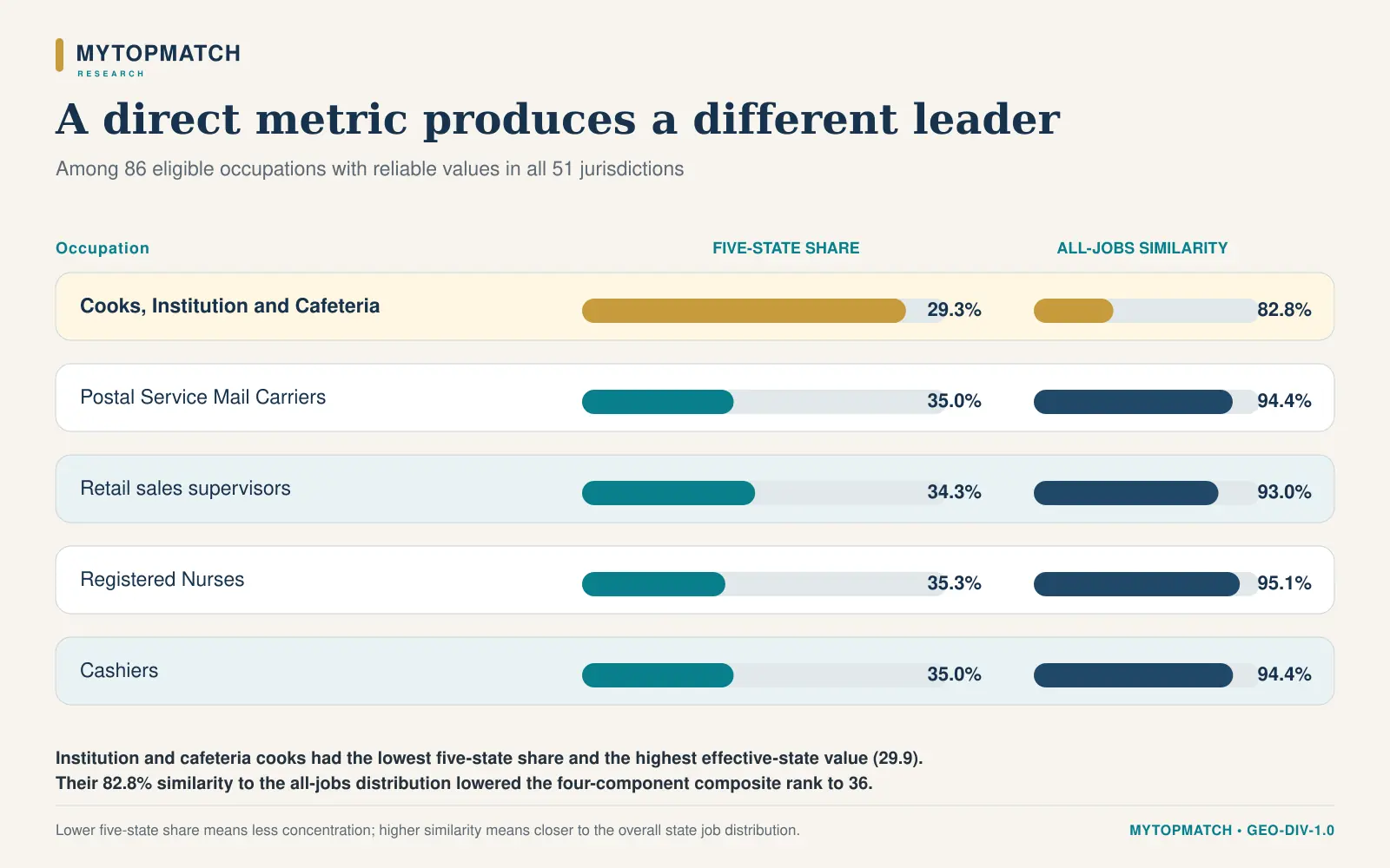
Composite rankings can conceal tradeoffs. Among the 86 eligible occupations with reliable values in all 51 jurisdictions, Cooks, Institution and Cafeteria had the lowest five-state share, 29.3%, and the highest effective-state value, 29.9.
That occupation ranked 36th on the composite because its state employment pattern was less similar to the overall all-jobs distribution, at 82.8%. This contrast is useful. An occupation can be distributed unusually evenly across states without closely tracking where employment overall is located.
MyTopMatch therefore recommends using the component columns as well as the composite. A worker who values a flatter state distribution may prefer the direct concentration measures. A workforce planner who wants an occupation to follow the national employment footprint may emphasize the all-jobs similarity component.
Suppressed estimates are missing, not zero
BLS explains that an occupation-area estimate may be withheld because it fails quality standards or because publication could compromise respondent confidentiality. When neither employment nor wage can be published, the occupation may not appear in the area data at all. [5]
Article 11 never converts an absent or withheld state cell to zero employment. The primary cell rule requires a published total-employment estimate and a published employment PRSE no greater than 20%. The headline universe then requires:
- national employment of at least 100,000;
- at least 45 reliable state/DC cells; and
- a sum of reliable state employment between 80% and 120% of the independently published national employment estimate.
The last range is a diagnostic, not an accounting identity. State and national estimates are published at different aggregation levels and are rounded. The band screens out distributions dominated by missing or inconsistent coverage without pretending the estimates must add exactly.
Of the 829 detailed or most-detailed occupation categories with at least one state/DC row, 234 passed all three headline gates. Eighty-six of those had reliable values in all 51 jurisdictions. Prosthodontists appeared in the national detailed file but had no state/DC row; Article 11 treats that as unavailable state evidence, not as zero employment.
What workers can learn from the results
The robust tier can help a worker ask better location questions:
- How dependent is this occupation on a few states? A broad footprint can provide more state-level options if a worker needs or wants to move.
- Where inside the state are the jobs? State breadth can coexist with strong metro, rural, hospital, school, government, or employer concentration.
- What does the local market pay? Article 11 does not combine diversification with wages or living costs. Those questions belong to the separate Geographic Opportunity study.
- Are there current openings? Existing employment is not a vacancy count. Current employer demand requires separate, timely evidence.
- Can the worker legally and practically enter? Licensing, certification, education, experience, working conditions, and employer requirements remain separate.
Geographic diversification is best understood as one form of career optionality. It can reduce exposure to a single place while leaving other risks unchanged.
What employers and workforce organizations can learn
For employers, a broad occupation footprint may support multi-state recruiting and benchmarking, but it does not guarantee an adequate local supply. The useful next checks are local concentration, compensation, commuting patterns, licensing, and actual applicant flow.
For workforce organizations, the analysis can identify occupations whose training pathways may be relevant across many states. Before scaling a program, organizations should examine state and local requirements, placement outcomes, employer partnerships, and occupation-specific demand.
For policymakers, the findings provide a descriptive map of where existing employment is distributed. They do not identify labor shortages, prove that workers can move freely between states, or estimate the effects of a training or licensing policy.
What the study cannot establish
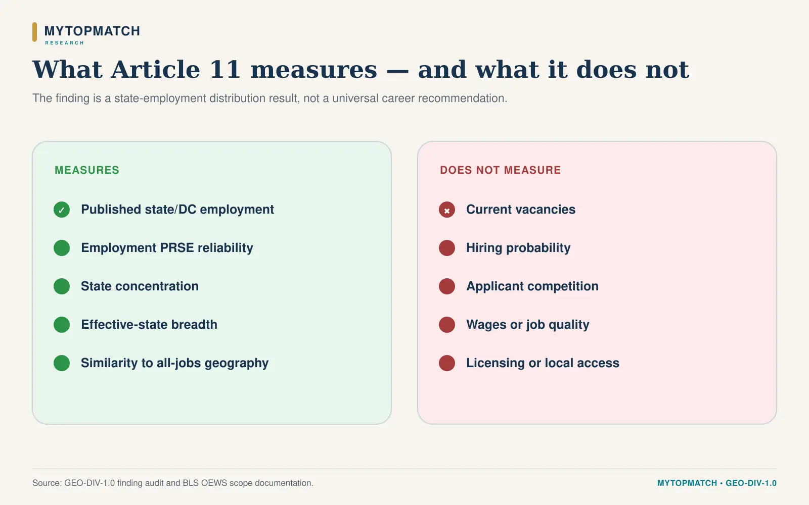
Article 11 cannot establish:
- current vacancies or advertised job counts;
- the probability that an applicant will be hired;
- employment in every city, county, or rural area within a state;
- wage attractiveness, purchasing power, benefits, schedules, or working conditions;
- historical resilience or future stability;
- individual relocation outcomes;
- legal access, licensing portability, or employer-specific requirements; or
- causal effects of geographic diversification on wages, unemployment, or career success.
The results are point-in-time, state-level descriptive estimates. A future annual series can test whether the tier persists across releases, but Article 11 does not use the word “stable” to describe change over time.
Methodology
Source release and freshness
As of the September 8, 2026 analysis freeze, the BLS OEWS tables page listed May 2025 as the current annual release and provided national and state downloadable files. The page was last modified May 15, 2026. [1]
Article 11 acquired:
- oesm25st.zip, SHA-256 74d5be0e1df865517d22dc3bd1fc3a8af5f6f9e3052a2163143021505d8e04c6; and
- oesm25nat.zip, SHA-256 b5855a37f3e03e779f6fbf173d3bbc94aeeff33426aef32fa95ce6d025bab1af.
The files are preserved unchanged in the internal raw-data layer. Transformed analytical copies and scripts are versioned separately.
OEWS scope
BLS describes OEWS as an employer survey measuring occupational employment and wage rates for wage-and-salary workers in nonfarm establishments. The May 2025 estimates use six semiannual panels collected from November 2022 through May 2025. The survey excludes self-employed workers, owners and partners in unincorporated firms, household workers, unpaid family workers, and most agriculture. [4]
Article 11 uses cross-industry state and national employment estimates only. It retains the 50 states and the District of Columbia and excludes Puerto Rico, Guam, and the U.S. Virgin Islands from the primary geography.
Occupational scope
The analysis selects rows that OEWS designates detailed. BLS notes in the downloadable field description that, for occupations no longer published at the SOC detailed level, this designation may represent the most detailed available broad occupation or an OEWS-specific combination. The supporting workbook preserves the published code and title and does not silently map these rows to another taxonomy.
Cell eligibility
A primary state cell is usable when:
published total employment is numeric AND published employment PRSE <= 20
The state file defines total employment as estimated employment rounded to the nearest ten and excluding self-employed workers. It defines PRSE as model error expressed as a percentage of the estimate, with lower values typically indicating greater precision in the presence of model error. The 20% ceiling is a MyTopMatch quality rule, not a threshold endorsed by BLS.
Occupation eligibility
An occupation enters the headline universe when:
national employment >= 100,000
reliable state/DC count >= 45
0.80 <= reliable state employment sum / national employment <= 1.20
No value is imputed. Occupations that fail a gate remain in the all-occupation analytical output with an explicit status but are excluded from headline ranking.
Component formulas
For occupation o and reliable jurisdictions j, let s_oj be jurisdiction j's share of the occupation's reliable-state employment.
five-state share = sum of the five largest s_oj values
HHI = sum over j of s_oj squared
effective states = 1 / HHI
Let a_j be jurisdiction j's share of all-occupation employment across the same observed jurisdictions.
all-jobs similarity = 1 - 0.5 x sum over j of |s_oj - a_j|
Reliable-state coverage, effective states, inverse five-state share, and all-jobs similarity are percentile-ranked within the 234-occupation headline universe. Higher percentiles always indicate greater diversification.
Geographic Diversification Score = mean of the four component percentiles
Robust-tier rule
An occupation qualifies for the robust tier only if it is top ten in:
- the primary PRSE <=20%, 50-state-plus-DC specification;
- the PRSE <=15% specification;
- the PRSE <=25% specification; and
- the 50-state specification excluding DC;
and it must appear in the top ten in at least 90% of 2,000 component-weight draws.
For each draw, the four equal weights receive independent multipliers sampled from Uniform(0.5, 1.5), then are renormalized to sum to one. The random seed is 20260908. Results are sensitivity summaries conditional on this design.
Validation
- Preserved and hashed both official source ZIP files.
- Confirmed 51 retained state/DC jurisdictions and one all-occupation row per jurisdiction.
- Confirmed 35,223 detailed or most-detailed occupation-state rows in the retained geography.
- Confirmed 830 national rows designated detailed and 829 corresponding categories with state/DC evidence.
- Recalculated the four tier members' state counts, five-state shares, effective-state values, and all-jobs similarities directly from the official source files.
- Rebuilt the full ranking under three alternate cell/geography specifications.
- Tested 2,000 weight draws with a frozen seed.
- Applied leave-one-component-out checks and preserved their ranks in the supporting workbook.
- Retained source, derived, robustness, interpretation, and non-claim categories in a claim ledger.
Limitations
- Employment is not hiring. OEWS employment stocks do not count current openings, postings, applicants, or offers.
- State is a broad geography. Jobs may be concentrated in particular metros, facilities, institutions, or rural areas.
- Survey universe. The self-employed and several other worker classes are excluded; most agriculture is outside OEWS coverage. [4]
- Three-year panel design. May 2025 estimates combine six panels and are not a single-month census. [4]
- Suppression. Missing state cells can reflect confidentiality or quality rules. They are never interpreted as zero. [5]
- Analyst-defined thresholds. National employment, reliable-state count, coverage ratio, and PRSE cutoffs are MyTopMatch rules.
- Composite dependence. Rankings depend on component definitions, normalization, and weights; the robust tier reduces but does not eliminate that dependence.
- Rounded employment. Published total-employment values are rounded to the nearest ten.
- Point-in-time edition. The study does not establish time-series persistence or future resilience.
- No causal claim. The analysis cannot show that geographic diversification causes better worker outcomes.
Adversarial validation: how could this result be wrong?
The tier could be misleading if suppressed cells were mistaken for absence, if state and national estimates were treated as exact accounting totals, if a single composite specification drove the result, if large-state population patterns were confused with even geographic distribution, or if existing employment were interpreted as vacancies.
Article 11 addresses those risks by retaining missing cells, requiring broad reliable coverage, screening state-to-national coverage, publishing direct concentration metrics, adding all-jobs similarity, testing thresholds and geography, perturbing component weights, and using a non-claim boundary. Remaining risks are stated above rather than converted into false precision.
Finding audit record
FINDING ID: MTM-GEO-002 STUDY: Occupational Geographic Diversification RESEARCH QUESTION: Which large occupations have the most broadly and robustly distributed state-level wage-and-salary employment? DATA SOURCES: BLS OEWS May 2025 national and state downloadable files DATA RELEASE / VERSION: May 2025 OEWS; source page last modified May 15, 2026 DATE RANGE: May 2025 reference edition; six survey panels from November 2022 through May 2025 SAMPLE: 35,223 detailed or most-detailed occupation-state rows; 829 state-observed occupation categories; 234 headline-eligible occupations; 86 with reliable estimates in all 51 jurisdictions VARIABLES: State, occupation code/title, total employment, employment PRSE, national employment, all-occupation state employment CALCULATION: Coverage, top-five share, inverse HHI, all-jobs distribution similarity, percentile components, equal-weight composite, alternate specifications, weight draws STATISTICAL METHOD: Descriptive distribution analysis and deterministic sensitivity testing; no causal or inferential model RESULT: Postal Service Mail Carriers, First-Line Supervisors of Retail Sales Workers, Registered Nurses, and Cashiers formed the robust top-ten tier EFFECT SIZE: Five-state share 34.3%-35.3%; effective states 24.4-24.8; all-jobs similarity 93.0%-95.1% CONFIDENCE INTERVAL: Not calculated; PRSE is used as a cell-screening measure and is not converted into an index confidence interval ROBUSTNESS TESTS: PRSE ceilings of 15%, 20%, and 25%; DC exclusion; 2,000 component-weight draws; leave-one-component-out ranks ALTERNATIVE EXPLANATIONS: State population and total employment size; government and institutional structure; industry location; suppression; regional demand; establishment distribution KNOWN LIMITATIONS: OEWS universe and panel design; state aggregation; suppression; point-in-time data; analyst-defined index choices; no vacancy or individual-access evidence CONFIRMATORY OR EXPLORATORY: CONFIRMATORY under the frozen GEO-DIV-1.0 rules; direct-metric cook result is a predefined component finding MODEL INTERPRETATION: Geographic distribution of existing state-level employment, not hiring access or career quality VALIDATION STATUS: PASSED FOR DESCRIPTIVE PUBLICATION PUBLICATION STATUS: PUBLISHED — WEBSITE ONLY
FAQ
Does this mean these occupations are hiring everywhere?
No. The study measures existing employment estimates. It does not observe current vacancies or recruiting activity.
Does a reliable estimate in a state mean jobs exist in every part of that state?
No. A state estimate can conceal substantial local concentration. Metro and nonmetro analysis is required for local claims.
Why include an all-jobs similarity measure?
A purely even distribution can reward occupations that are disproportionately represented in smaller states. The similarity component asks whether an occupation follows the broad distribution of employment overall. It is published beside the flatter-distribution metrics because neither construct should silently replace the other.
Why not rank all 829 state-observed occupation categories?
Many smaller or geographically concentrated occupations have too few reliable state cells for a defensible concentration comparison. The 234-occupation headline universe requires scale, coverage, and a state-to-national diagnostic.
Is the primary score an official BLS measure?
No. BLS publishes the source estimates. MyTopMatch defines the derived metrics, normalization, eligibility gates, score, and robust-tier rule.
Can the results be cited as original MyTopMatch research?
Third parties may describe the calculations and analysis as MyTopMatch original research while identifying BLS as the original data publisher and linking to the canonical MyTopMatch article.
Citation and reuse
Suggested citation: MyTopMatch Research. (2026). “Four Occupations Had the Most Robust State Employment Footprints.” MyTopMatch. https://mytopmatch.com/publications/careers-broadest-state-employment-footprints
When reusing findings, identify the work as original analysis by MyTopMatch Research, identify the underlying public data publisher where relevant, and link to this canonical article. Source publishers do not endorse MyTopMatch's calculations or interpretations.